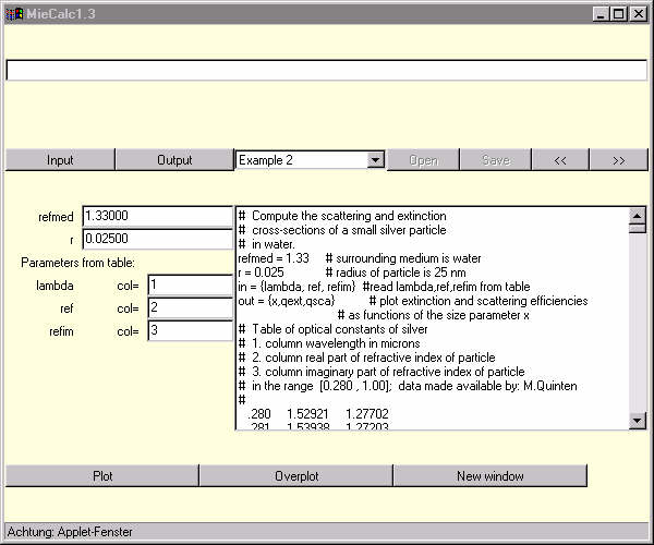
In example 2, we study the spectral dependence of the extinction and scattering efficiencies of silver particles. The optical constants (real and imaginary parts of the refractive index) change with wavelength (dispersion) and must be read in from a table given in the text area of the MieCalc's main window.
The parameter panel looks different from example 1. The parameters to
be read from the table are listed separately.
"col= 1" means that the respective parameter shall be
read from column 1 of the table. Click on "Plot" to obtain a beautiful
surface-plasmon resonance ....
Now change refmed in the text field on the right side of the parameter panel from 1.33 to 1.5 and click on "Overplot" to see how the surface-plasmon resonance looks like for silver embedded in glass..
More interested in angular scattering? Select the example "Angular scattering" which is a little bit more time consuming. In this example, the scattered irradiance is computed as a function of scattering angle theta. Three cases are studied:
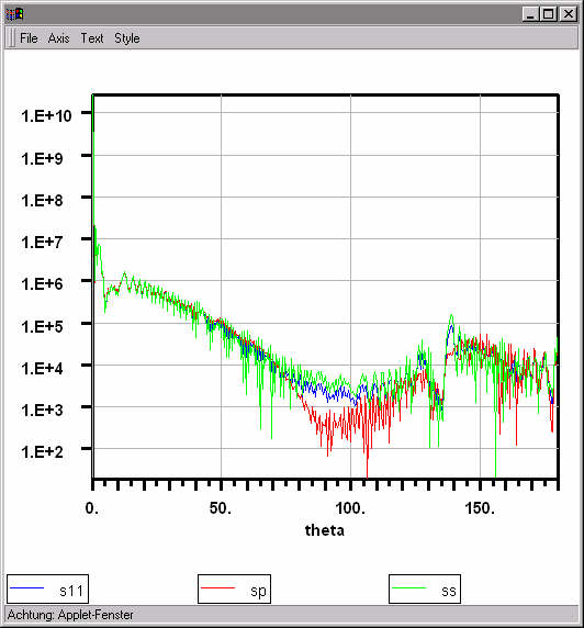
Note the feature at ca. 135-140 degrees. It's the rainbow angle! As you can see, polarization effects play an important effect for larger scattering angles, and are almost negligible in forward direction ("Fraunhofer diffraction").
Now, after having got an impression about the capabilities of MieCalc,
you should study the documentation to learn
more details.