USER GUIDE
<<<< BACK

Plotting data

1.  your internet browser.
2. the number of data points
3. the size parameter x of the sphere. For x >> 10, the computation time increases approximately linearily with x.

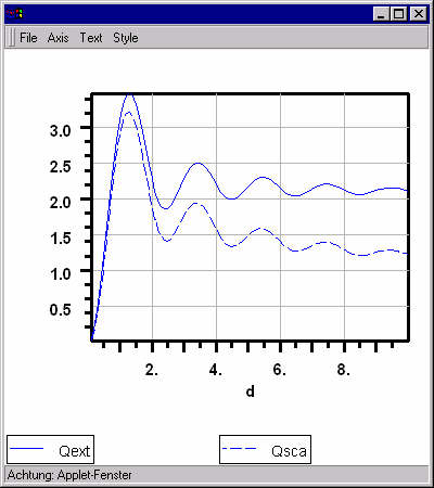
For this result, the following values for the input parameters have been choosen:  lambda=0.5 refmed=1.33, ref=1.58, refim=0.01, and d is varied from 0.01 to 10 using 100 datapoints. Change the value of  refmed to 1.0 to see how the same particle "behaves" in air instead of water. Click on   to "add" the result to the previous plot:

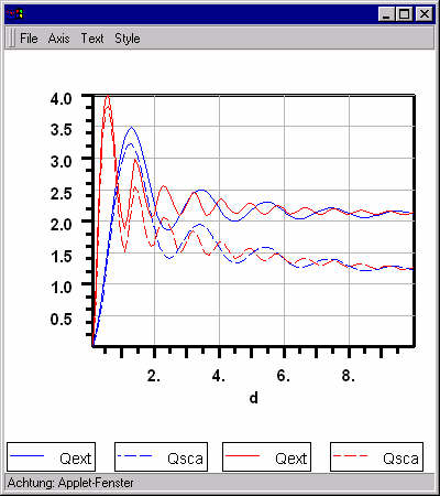
The curves in red show the results of the second calculation. Click on the labels , , , or  to open a dialog box in which you can modify style, color, line thickness and label text of the corresponding plot. Use the menu "Axis" of the plot window to change between linear and logarithmic scaling of the plot or to specify upper and lower bounds for the coordinates. Simply try out (the "a" in the dialog for the coordinate bounds means automatic, i.e, the bound is calculated from the data).  Use the menu "Text" to set/modify the  titles for the x-axis, y-axis and the overall title. The menu "Style" can be used to change the style of the grid (no grid, coarse grid, fine grid) . Most entries of the  menu "File", finally, are disabled in the internet version. In the stand alone version  of MieCalc, you can use this menu to print the plot, convert it into encapsulated Postscript, or to save the result  in ASCII-format.  Click here, to learn more about the functional elements of the plot window.

In contrast to "Overplot",  clicking on "Plot" erases the previous plot (if there was any) and "New Window" opens an additional plot window.

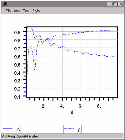
As an example, open the output dialog by clicking on ,  de-select  Qext and Qsca   and select   g - the asymmetry parameter and A - the albedo. Close the output dialog. Now click on  to obtain the following plot in a new window:

 

CONTINUE >>>>